神经网络
神经网络可以通过使用torch.nn包进行构建
现在你粗略了解了autograd,nn依赖autograd去定义模型还有求微分。一个nn.Module含有很多层和forward(input)方法,forward方法返回output
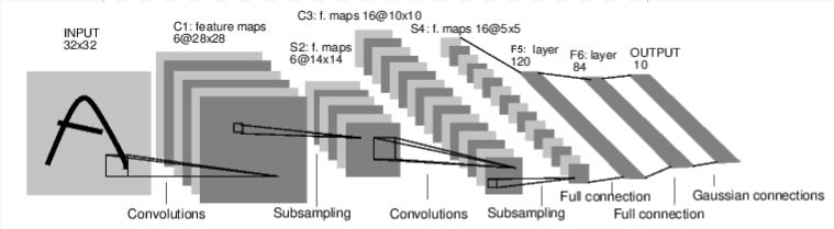
这是一个前馈网络的例子。他接收输入,逐层传递输入,最终给出输出
一个典型的神行网络训练流程如下:
- 定义有一些可学习参数的神经网络
- 遍历输入的数据集
- 通过网络处理输入
- 计算损失(输出和正确解有多远)
- 将梯度传回网络参数中
- 更新网络权重, 经典的更新例子: W = W - lr * grad
定义网络
1 | import os |
out:
Net(
(conv1): Conv2d(1, 6, kernel_size=(5, 5), stride=(1, 1))
(conv2): Conv2d(6, 16, kernel_size=(5, 5), stride=(1, 1))
(fc1): Linear(in_features=400, out_features=120, bias=True)
(fc2): Linear(in_features=120, out_features=84, bias=True)
(fc3): Linear(in_features=84, out_features=10, bias=True)
)
你仅仅是需要定义forward方法,backward方法(计算梯度)是自动定义好的。你可以使用任何操作在forward方法中。
学习的模型参数由net.parameters()返回。
1 | params = list(net.parameters()) |
10
torch.Size([6, 1, 5, 5])
尝试随机32x32输入,注意:预期的输入这个网络(LeNet)的输入时32x32的。用MNIST数据集在这个网络上的话,请将图像尺寸改为32x32
1 | input = torch.randn(1, 1, 32, 32) |
out:
tensor([[-0.0771, 0.0865, 0.1370, 0.1146, -0.0952, -0.0172, -0.0014, -0.0123,
0.0449, 0.1213]], grad_fn=
所有参数的梯度缓存清零。然后随机梯度传播
1 | net.zero_grad() |
Note:
torch.nn 仅支持mini-batches。 整个torch.nn包仅支持输入一个样本的mini-batch,而不是单个样本
比如,nn.Conv2d将收到(nSamples x nChannels x Height x Width)的4D(4维张量)。
如果你有一个样本,就用input.unsqueeze(0)去添加一个假的批维度(batch dimensioin)
损失函数
一个损失行数有(output, target)两部分的输入,计算输出和目标有多远。
nn包中的loss function有一点不同。 一个简单的loss是:nn.MSELoss,它计算的是输入和目标的均方差
如:
1 | output = net(input) |
out:
tensor(0.7784, grad_fn=
现在,如果你跟着loss的方向走,用它的.grad_fn属性,你会看到一个计算图
1 | input -> conv2d -> relu -> maxpool2d -> conv2d -> relu -> maxpool2d |
所以,当我们调用loss.backward(), 整个图是分化为w.r.t神经网络的参数,然后所有在图中有requires_grad=True的张量会有他们的.grad,Tensor累计的梯度。
为了证明,我们退几步
1 | print(loss.grad_fn) # MSELoss |
out:
反向传播
反向传播误差,我们所需要做的就是loss.backward(). 你需要清理掉已存在的梯度,否则会被累加到存在的梯度上。
现在我们尝试调用loss.backward(),观察在backward前后的conv1的偏置梯度
1 | print('conv1.bias.grad before backward') |
out:
conv1.bias.grad before backward
None
conv1.bias.grad after backward
tensor([ 8.4313e-05, 5.5547e-03, 1.2019e-02, 4.9749e-03, -9.5904e-05,
2.6212e-03])
更新权重
最简单的在训练中更新规则是随机梯度下降(SGD):
1 | weight = weight - learning_rate * gradient |
我们可以通过简单的python代码实现
1 | learning_rate = 0.01 |
然而,由于你使用的神经网络,你想使用各种不同的更新规则例如,SGD, Nesterov-SGD,Adam,RMSProp等等。我们构建了一个小包:torch.optim用来实现所有的这些方法。
1 | # 创建优化器 |