本文最后编辑于
误差反向传播法 计算图 计算图:将计算过程用图形表达出来。
首先说下书上的例子:
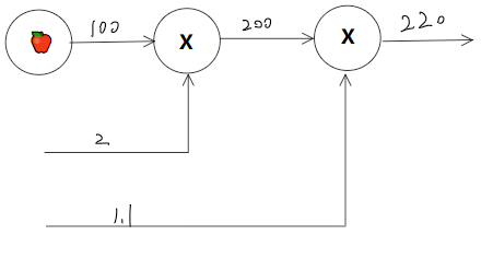
问题1: 太郎在超市买了2个100日元一个的苹果,消费税是10%,请计算支付金额。
相当简单的一道题, 2 100 1.1即可。计算图表示则是:
将x2和x1.1节点中的数字取出,符号单独放在○当中。
这种从左往右的计算方式为正向传播
从右往左的计算方式则是反向传播
局部计算 简单来说就是只用关注当前的简单计算部分,其他复杂的部分不需要管。意思就是计算偏导的那种感觉。
为何用计算图解题 优点:
局部计算,无论全局是多么复杂,都可以通过局部计算使各个节点致力于简单计算,简化问题。
可以将中间的计算结果全部保存起来。
通过反向传播高效计算导数。
基于反向传播的导数的传递
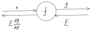
计算图的反向传播 先看一个
就是将信号E乘以节点的局部导数,然后传递到下一个节点。如果假设y = x^2 那么导数为2x,那么向下传播的值就是 E*2x,这里的x是正向传递时记录的。
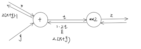
链式法则
就是高数里对复合函数求导。
e.g令 链式法则和计算图
反向传播 对于每个层,都有forward方法和backward方法,对应正向反向传播。在训练时创建网络时,将每一层存在一个列表当中,顺序正向传播。当需要计算梯度时,将列表翻转,依次执行backward方法进行反向传播,求得梯度。
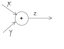
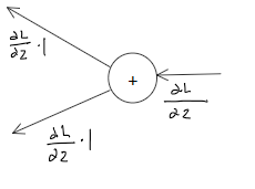
加法节点的反向传播 正向计算图
此处是 z = x + y,分别对x,y求偏导。结果都是1。按照前面说的反向传播的话就是将前面给的E乘上局部的导数可知,对于加法来说,都是将E*1传给后面。
python实现:
1
2
3
4
5
6
7
8
9
class AddLayer : def __init__ (self ): pass def forward (self,x,y ): return (x + y) def backward (self,dout ): dy = dout * 1 dx = dout * 1 return dx,dy
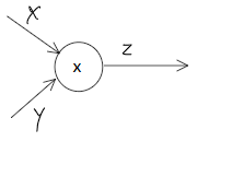
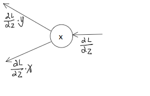
乘法节点的反向传播 考虑 f = xy的导数公式
反向传播图
由图中可知对于乘法,是将E乘上输入信号的翻转值。
python实现:
1
2
3
4
5
6
7
8
9
10
11
12
13
14
class MulLayer : def __init__ (self ): self.x = None self.y = None def forward (self,x,y ): self.x = x self.y = y out = x * y return out def backward (self,dout ): dx = dout * self.y dy = dout * self.x return dx,dy
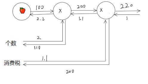
回到苹果的例子 对于买苹果的例子反向传播则是
首先最终结果是220,导数就是1,向后传播,是一个乘法传播,E乘上输入信号的翻转值,也就是200和1.1交换相乘,得到1.1和200。继续向后传播,也是乘法,交换相乘得到2.2和110。
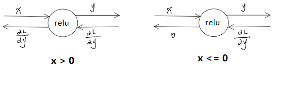
激活函数层实现 ReLU层 数学公式:
python实现:
1
2
3
4
5
6
7
8
9
10
11
12
13
class Relu : def __init__ (self ): self.mask = None def forward (self,x ): self.mask = (x <= 0 ) out = x.copy() out[self.mask] = 0 return out def backforward (self,dout ): dout[self.mask] = 0 dx = dout return dx
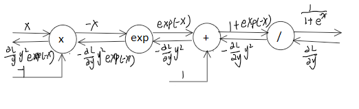
sigmoid层 数学公式
python实现:
1
2
3
4
5
6
7
8
9
import numpy as npclass sigmoid : def __init__ (self ): self.out = None def forward (self,x ): self.out = 1 / (1 + np.exp(-x)) return self.out def backward (self,dout ): dx = dout * (1.0 - self.out) * self.out
Affine/Softmax 层 Affine层:
就是原先乘上权重加上偏置的操作,对于矩阵的正向反向传播
python实现
1
2
3
4
5
6
7
8
9
10
11
12
13
14
15
16
17
18
19
20
21
22
23
import numpy as npclass Affine : def __init__ (self,W,b ): self.W = W self.b = b self.x = None self.original_x_shape = None self.dW = None self.db = None def forward (self,x ): self.original_x_shape = x.shape x = x.reshape(x.shape[0 ], -1 ) self.x = x out = np.dot(self.x, self.W) + self.b return out def backforward (self,dout ): dx = np.dot(dout,self.W.T) self.dW = np.dot(self.x.T,dout) self.db = np.sum (dout,axis=0 ) dx = dx.reshape(*self.original_x_shape) return dx
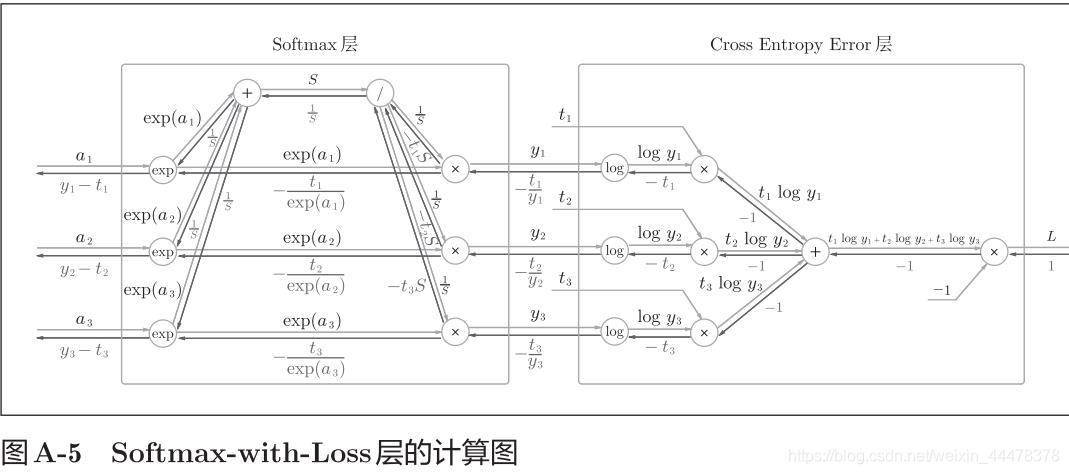
Softmaxwithloss层
python实现
1
2
3
4
5
6
7
8
9
10
11
12
13
14
15
16
17
18
19
20
21
22
23
24
25
26
27
28
29
30
31
32
33
34
35
36
37
38
39
40
41
42
import numpy as npclass SoftmaxWithLoss : def __init__ (self ): self.loss = None self.y = None self.t = None def softmax (self,x ): if x.ndim == 2 : x = x.T x = x - np.max (x, axis=0 ) y = np.exp(x) / np.sum (np.exp(x), axis=0 ) return y.T x = x - np.max (x) return np.exp(x) / np.sum (np.exp(x)) def cross_entropy_error (self,y, t ): if y.ndim == 1 : t = t.reshape(1 , t.size) y = y.reshape(1 , y.size) if t.size == y.size: t = t.argmax(axis=1 ) batch_size = y.shape[0 ] return -np.sum (np.log(y[np.arange(batch_size), t] + 1e-7 )) / batch_size def forward (self,x,t ): self.t = t self.y = self.softmax(x) self.loss = self.cross_entropy_error(self.y,self.t) return self.loss def backforward (self,dout = 1 ): batch_size = self.t.shape[0 ] if self.t.size == self.y.size: dx = (self.y - self.t) / batch_size else : dx = self.y.copy() dx[np.arange(batch_size), self.t] -= 1 dx = dx / batch_size return dx