本文最后编辑于 前,其中的内容可能需要更新。
神经网络的学习
这章主要讲的是函数斜率的梯度法
计算机视觉领域常用的特征量包括 SIFT、SURF、HOG等。
训练数据和测试数据
训练数据和测试数据 : 首先使用训练数据进行学习,寻找最优的参数,然后使用测试数据评价训练得到的模型的实际能力。
为了正确评价模型的泛化能力,就必须划分训练数据和测试数据。训练数据又称为监督数据。
过拟合:只对某个数据集过度拟合的状态。
损失函数
损失函数:表示神经网络性能的“恶劣程度”的指标,当前神经网络对监督数据再大多成都上不拟合,大多程度不一致。通常乘上一个负值,解释为“多大程度上不坏”,“性能上有多好“。 损失函数可以用任何函数,不过一般都用的均方误差或交叉熵
个人理解:就是神经网络的预测与实际的标签,相差距离的多少。
均方误差
公式:
yk : 神经网络的输出
tk : 监督数据
k : 数据维数
python表示:
1
2
| def mean_squared_error(y,t):
return 0.5 * np.sum((y - t)**2)
|
拿MNIST数据做一次尝试
假设:
预测数据 [0.1,0.05,0.6,0.0,0.05,0.1,0.0,0.1,0.0,0.0]
正确解(one_hot) [0,0,1,0,0,0,0,0,0,0] #正确解为2
1
2
3
4
5
6
7
8
9
10
11
12
| y = np.array([0.1,0.05,0.6,0.0,0.05,0.1,0.0,0.1,0.0,0.0])
t = np.array([0,0,1,0,0,0,0,0,0,0])
def mean_squared_error(y,t):
    return 0.5 * np.sum((y - t)**2)
y2 = np.array([0.1,0.05,0.1,0.0,0.05,0.1,0.0,0.6,0.0,0.0])
print(mean_squared_error(y,t))
print(mean_squared_error(y2,t))
|
out:
0.09750000000000003
0.5975
很明显显示第一个例子与监督数据更加吻合。
交叉熵误差
公式:
符号解释,同上面
由于tk中只有正确解为1,其他为0,所以只用计算正确解标签的输出的自然对数。因此可知,交叉熵误差的值是由正确解标签所对应的输出的结果决定的
python实现:
1
2
3
| def cross_entropy_error(y,t):
delta = 1e-7
return -np.sum(t * np.log(y + delta)) / y.shape[0]
|
同样拿之前的假设做对比
1
2
3
4
5
6
7
8
9
10
|
def cross_entropy_error(y,t):
delta = 1e-7
return -np.sum(t * np.log(y + delta)) / y.shape[0]
print(cross_entropy_error(y,t))
print(cross_entropy_error(y2,t))
|
out:
0.0510825457099338
0.23025840929945457
mini-batch学习
在机器学习使用训练数据进行学习,需要针对训练数据计算损失函数值,找出使这个值尽可能小的参数。计算损失函数的时候需要将所有训练数据作为对象。也就是说,如果有100个训练数据,需要把100个的损失函数的总和作为学习的指标。
以交叉熵为例:
就只是把单个的损失函数数据扩大到了N份,最后还是需要除以N做一次正规化。就是求的“平均损失函数”。对于MNIST数据集有60000个训练数据,不可能每个都加上,这样花费的时间较多。因此会从中随机选择100笔,再用100笔数据进行学习。这就是mini-batch学习
python实现
1
2
3
4
5
6
7
8
9
| import numpy as np
from mnist import load_mnist
(x_train,t_train),(x_test,t_test) = load_mnist(normalize=True,one_hot_label=True)
train_size = x_train.shape[0]
batch_size = 10
batch_mask = np.random.choice(train_size,batch_size)
x_batch = x_train[batch_mask]
t_batch = t_train[batch_mask]
|
np.random.choice() 从指定的数字中随机选择想要的数字。
mini-batch交叉熵的实现
1
2
3
4
5
6
7
| def cross_entropy_error(y,t):
if y.ndim == 1:
t = t.reshape(1,t.size)
y = y.reshape(1,y.size)
batch_size = y.shape[0]
return -np.sum(t * np.log(y + 1e-7)) / batch_size
|
另一种实现
1
2
3
4
5
6
7
8
9
10
11
| def cross_entropy_error(y, t):
if y.ndim == 1:
t = t.reshape(1, t.size)
y = y.reshape(1, y.size)
if t.size == y.size:
t = t.argmax(axis=1)
batch_size = y.shape[0]
return -np.sum(np.log(y[np.arange(batch_size), t] + 1e-7)) / batch_size
|
设定损失函数原因
为什么不以精度为指标?
为了使损失函数的值尽可能小,需要计算参数的导数(梯度),以导数为指引,逐步更新参数值。
对权重参数的损失函数求导,表示对如果稍微改变这个权重的值,损失函数的值该如何变化。
如果为负: 通过改变权重向正方向改变,即可减小损失函数的值。
如果为正: 通过改变权重向负方向改变,即可减少损失函数的值。
如果用精度作为指标,大多数地方导数变为0,无法更新。
数值微分
导数
就和高数讲的一样
1
2
3
4
| import numpy as np
def numerical_diff(f,x):
h = 1e-4
return (f(x + h) - f(x - h)) / (2 * h)
|
偏导
也是和高数一样
假设公式:
偏导
梯度
梯度:由全部变量的偏导汇总而成的向量
e.g
python实现也很简单
1
2
3
4
5
6
7
8
9
10
11
12
13
14
15
16
17
18
| import numpy as np
def numerical_gradient(f,x):
h = 1e-4
grad = np.zeros_like(x)
for idx in range(x.size):
tmp_val = x[idx]
x[idx] = tmp_val + h
fxh1 = f(x)
x[idx] = tmp_val - h
fxh2 = f(x)
grad[idx] = (fxh1 - fxh2) / (2 * h)
x[idx] = tmp_val
return grad
|
梯度法
梯度法:通过不断地沿梯度方向前进逐渐减小函数值的过程
寻找最小值是梯度下降法,寻找最大值是梯度上升法
数学表达:
其中η是更新量,在机器学习中是学习率
学习率是实现设定的值
1
2
3
4
5
6
| def gradient_descent(f,init_x,lr = 0.1, step_num = 100):
x = init_x
for i in range(step_num):
grad = numerical_gradient(f, x)
x -= lr * grad
return x
|
init_x 是初始值, lr是学习率,step_num 是重复次数
现在可以尝试求解 f(x0,x1) = x0^2 + x1 ^2 的最小值
1
2
3
4
5
6
7
8
9
10
11
12
13
|
def fun1(x):
return x**2 + 10
def fun2(x):
return x[0]**2 + x[1]**2
if __name__ == '__main__':
print('微分')
print(numerical_diff(fun1, 1))
print("梯度")
print(numerical_gradient(fun2, np.array([3.0,4.0])))
print('梯度下降法求 f(x0,x1) = x0^2 + x1^2 最小值')
print(gradient_descent(fun2, np.array([-0.3,4.0])))
|
out:
微分
2.0000000000042206
梯度
[6. 8.]
梯度下降法求 f(x0,x1) = x0^2 + x1^2 最小值
[-6.11110793e-11 8.14814391e-10]
结果是十分接近(0,0)点,而事实上最低点就是(0,0)点
学习率这样的参数称为超参数。它和权重参数是不同的,权重是可以通过数据和学习自动获得的。学习率这样的超参数是人工设定的。
2层神经网络的类
通过梯度下降法更新参数,由于数据是随机选择的mini batch数据,又称之为随机梯度下降法(stochastic gradient descent)简称SGD
写一个名为TwoLayerNet类
1
2
3
4
5
6
7
8
9
10
11
12
13
14
15
16
17
18
19
20
21
22
23
24
25
26
27
28
29
30
31
32
33
34
35
36
37
38
39
40
41
42
43
44
45
46
47
48
49
50
51
52
53
54
55
56
57
58
59
60
61
62
63
64
| import numpy as np
class TwoLayersNet:
def __init__(self,input_size,hidden_size,output_size,weight_init_std = 0.01):
self.params = {}
self.params["W1"] = weight_init_std * np.random.randn(input_size,hidden_size)
self.params["b1"] = np.zeros(hidden_size)
self.params["W2"] = weight_init_std * np.random.randn(hidden_size,output_size)
self.params["b2"] = np.zeros(output_size)
def predict(self,x):
W1,W2 = self.params["W1"],self.params["W2"]
b1,b2 = self.params["b1"],self.params["b2"]
a1 = np.dot(x,W1) + b1
z1 = sigmoid(a1)
a2 = np.dot(z1,W2) + b2
y = softmax(a2)
return y
def loss(self,x,t):
y = self.predict(x)
return cross_entropy_error(y,t)
def accuracy(self,x,t):
y = self.predict(x)
y = np.argmax(y,axis=1)
t = np.argmax(t,axis=1)
accuracy = np.sum(y == t) / float(x.shape[0])
return accuracy
def numerical_gradient(self,x,t):
loss_W = lambda W: self.loss(x, t)
grads = {}
grads["W1"] = numerical_gradient(loss_W, self.params['W1'])
grads["W2"] = numerical_gradient(loss_W, self.params['W2'])
grads["b1"] = numerical_gradient(loss_W, self.params['b1'])
grads["b2"] = numerical_gradient(loss_W, self.params['b2'])
return grads
def gradient(self, x, t):
W1, W2 = self.params['W1'], self.params['W2']
b1, b2 = self.params['b1'], self.params['b2']
grads = {}
batch_num = x.shape[0]
a1 = np.dot(x, W1) + b1
z1 = sigmoid(a1)
a2 = np.dot(z1, W2) + b2
y = softmax(a2)
dy = (y - t) / batch_num
grads['W2'] = np.dot(z1.T, dy)
grads['b2'] = np.sum(dy, axis=0)
da1 = np.dot(dy, W2.T)
dz1 = sigmoid_grad(a1) * da1
grads['W1'] = np.dot(x.T, dz1)
grads['b1'] = np.sum(dz1, axis=0)
return grads
|
首先看__init__方法,input_size,hidden_size,output_size。依次表示的是输入层神经元数、隐藏层神经元数、输出层神经元数。input_size是784,因为输入的图像是(28x28)的,output_size也就是对应输出层,总共10个类型,所以是10。中间隐藏层是设定合适的值即可。书上设定的50个,我设定的100个,感觉效果比50的要好一点。权重使用的高斯分布的随机数进行初始化。
预测就是和之前的神经元一样,两层。乘上权重加上偏置,过一次sigmoid,然后进入二层,乘上权重加上偏置,过softmax,看概率。
损失函数,用的mini batch的交叉熵。
梯度下降,用的偏导,这个地方也是很耗时的,所以最终使用的时候用下边的gradient,使用的误差反向传播算法。
mini batch的实现
1
2
3
4
5
6
7
8
9
10
11
12
13
14
15
16
17
18
19
20
21
22
23
24
25
26
27
28
29
30
31
32
33
| import numpy as np
from mnist使用.mnist import load_mnist
from 两层神经网络的类 import TwoLayersNet
import matplotlib.pyplot as plt
import pickle
(x_train,t_train),(x_test,t_test) = load_mnist(normalize=True,one_hot_label=True,flatten = True)
train_loss_list = []
iters_num = 10000
train_size = x_train.shape[0]
batch_size = 100
learning_rate = 0.1
network = TwoLayersNet(input_size = 784, hidden_size = 100, output_size = 10)
for i in range(iters_num):
batch_mask = np.random.choice(train_size,batch_size)
x_batch = x_train[batch_mask]
t_batch = t_train[batch_mask]
grad = network.gradient(x_batch, t_batch)
for key in ('W1','b1','W2','b2'):
network.params[key] -= learning_rate * grad[key]
loss = network.loss(x_batch, t_batch)
train_loss_list.append(loss)
|
整个就是梯度下降实现了,先设定好超参数,循环10000次,每次循环都是随机抽取batch_size个训练数据,扔到梯度下降的函数中去。获得偏导的向量,然后依据偏导向量乘上学习率,一点点修改权值。最终查看loss_list会发现,损失值在不断减小。
基于测试数据的评价
这里引入一个新词
epoch : epoch是一个单位。一个epoch表示学习中所有训练数据均被使用过一次时更新数据。如10000个数据,用大小为100笔数据的mini batch训练学习时,重复SGD100次,所有的数据都被“看过”则是一个epoch。更正确的做法是,10000个数据全部打乱,然后100个一组训练,顺序训练100组。为一个epoch。
1
2
3
4
5
6
7
8
9
10
11
12
13
14
15
16
17
18
19
20
21
22
23
24
25
26
27
28
29
30
31
32
33
34
35
36
37
38
39
40
41
42
43
44
45
46
47
48
49
50
51
52
53
54
55
56
57
58
59
| import numpy as np
from mnist使用.mnist import load_mnist
from 两层神经网络的类 import TwoLayersNet
import matplotlib.pyplot as plt
import pickle
(x_train,t_train),(x_test,t_test) = load_mnist(normalize=True,one_hot_label=True,flatten = True)
train_loss_list = []
train_acc_list = []
test_acc_list = []
iters_num = 50000
train_size = x_train.shape[0]
batch_size = 100
learning_rate = 0.1
iter_per_epoch = max(train_size / batch_size,1)
network = TwoLayersNet(input_size = 784, hidden_size = 100, output_size = 10)
print(iter_per_epoch)
print(train_size)
for i in range(iters_num):
batch_mask = np.random.choice(train_size,batch_size)
x_batch = x_train[batch_mask]
t_batch = t_train[batch_mask]
grad = network.gradient(x_batch, t_batch)
for key in ('W1','b1','W2','b2'):
network.params[key] -= learning_rate * grad[key]
loss = network.loss(x_batch, t_batch)
train_loss_list.append(loss)
if i % iter_per_epoch == 0:
train_acc = network.accuracy(x_train, t_train)
test_acc = network.accuracy(x_test, t_test)
train_acc_list.append(train_acc)
test_acc_list.append(test_acc)
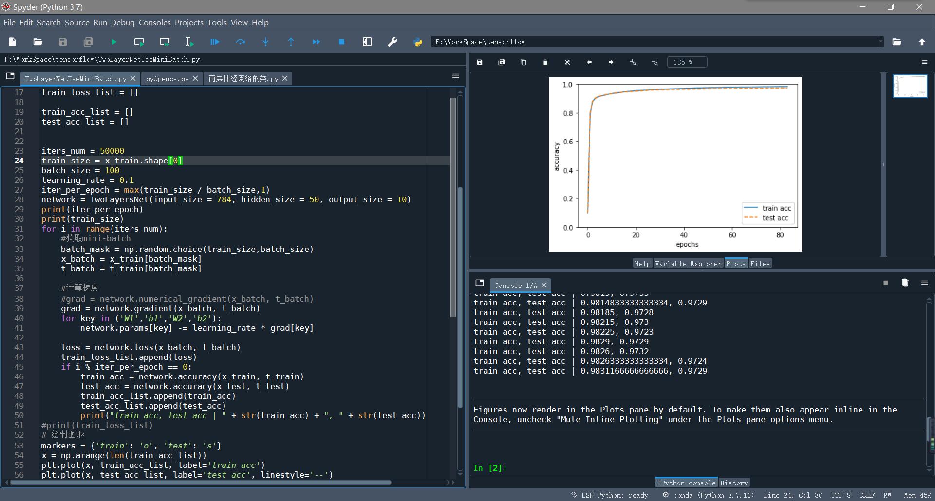
print("train acc, test acc | " + str(train_acc) + ", " + str(test_acc))
markers = {'train': 'o', 'test': 's'}
x = np.arange(len(train_acc_list))
plt.plot(x, train_acc_list, label='train acc')
plt.plot(x, test_acc_list, label='test acc', linestyle='--')
plt.xlabel("epochs")
plt.ylabel("accuracy")
plt.ylim(0, 1.0)
plt.legend(loc='lower right')
plt.show()
data_output = open('mnistData.pkl','wb')
pickle.dump(network, data_output)
data_output.close()
|
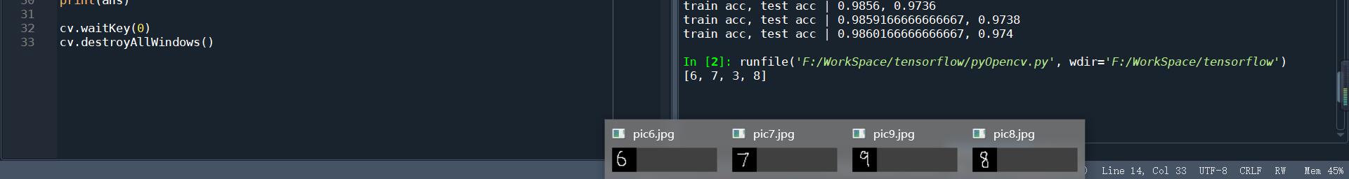
加了epoch的代码,后面有绘制图形。也有将训练好后将网络保存。方便随时读出,用opencv + numpy做识别手写数字。